NeuroAI for AI Safety
As AI systems become increasingly powerful, the need for safe AI has become more pressing. Humans are an attractive model for AI safety: as the only known agents capable of general intelligence, they perform robustly even under conditions that deviate significantly from prior experiences, explore the world safely, understand pragmatics, and can cooperate to meet their intrinsic goals. Intelligence, when coupled with cooperation and safety mechanisms, can drive sustained progress and well-being. These properties are a function of the architecture of the brain and the learning algorithms it implements. Neuroscience may thus hold important keys to technical AI safety that are currently underexplored and underutilized. In this roadmap, we highlight and critically evaluate several paths toward AI safety inspired by neuroscience: emulating the brain’s representations, information processing, and architecture; building robust sensory and motor systems from imitating brain data and bodies; fine-tuning AI systems on brain data; advancing interpretability using neuroscience methods; and scaling up cognitively-inspired architectures. We make several concrete recommendations for how neuroscience can positively impact AI safety.
Reverse-engineer sensory systems
Core idea
AI systems need robust sensory systems to be safe. Sensory systems in current AI systems are brittle: they are susceptible to adversarial examples [43], they learn slowly [62], they can fail catastrophically out-of-distribution [63], they tend to rely on shortcuts that generalize poorly [45], and they don’t display compositionality [64]. By contrast, sensory systems in the brain are robust [65]. If we could reverse engineer how sensory systems form these robust representations, we could embed them in AI systems, enhancing their safety. Sensory digital twins are large-scale neural networks trained to predict neural responses across a wide range of sensory inputs [66, 67, 68]. We evaluate reverse engineering the representations of sensory systems in model systems using sensory digital twins as an intermediate.
Why does it matter for AI safety and why is neuroscience relevant?
Adversarial robustness
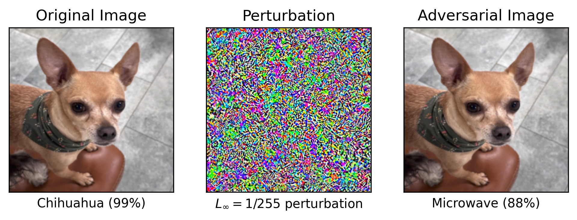
Adversarially crafted examples can cause AI systems to misbehave, and create an attack vector for malicious actors. Small perturbations to input data that are imperceptible to humans can cause otherwise highly capable models to make catastrophic errors in their predictions. While the most potent adversarial attacks leverage access to model internals, vulnerabilities still remain in the black-box setting [69]. Attackers can leverage decision-based boundary attacks, which iteratively adjust inputs based on model outputs to approximate decision boundaries in black-box settings [70]. These methods expose AI to vulnerabilities even without internal access, highlighting the risks of adversarial exploitation. Vulnerabilities of this kind have justifiably raised serious concerns, particularly at a time when AI systems are increasingly deployed in sensitive real-world contexts, including in autonomous settings [71].
The problem of adversarial robustness is not confined to any single domain of AI. Early results focused on image classification models, following the discovery that deep neural networks could be fooled through adversarial input perturbations [43], but similar vulnerabilities have been discovered in large language models [72] and in superhuman game-playing systems like KataGo [73]. Much effort has gone into developing more robust AI systems, and progress has been made through dedicated adversarial training. Scaling up models and datasets helps, but far less than one might hope. The most capable adversarially robust networks on CIFAR-10 and CIFAR-100 have required GPT-3.5-levels of compute to train, and still lag behind humans [47]. Scaling up adversarial robustness to human level on ImageNet is predicted to take multiple orders of magnitude compared to GPT-4. This has led to calls for preparing for a future where AI systems may remain inherently vulnerable to such attacks [74].
Adversarial robustness is a human phenomenon [45]: adversarial examples are defined by their inscrutability to humans, and it is natural to think that their solution may lie in studying the sensory systems of humans, and potentially primates and rodents. A potential framework to understand these issues [45] is in terms of robust and non-robust features. Both types of features are equally predictive in-distribution, but robust features remain predictive under varying amounts of distribution shift, unlike non-robust ones, which are highly sensitive to any such change. Since there are many more potential non-robust features than robust ones, deep neural networks are likely to exploit non-robust features as a result of their optimization process, which aims to maximize in-distribution performance. Biological perceptual systems are the result of an incomprehensibly large evolutionary search that has selected inductive biases to robustly generalize in real-world environments [75, 76].
Thus, adversarial robustness is an unsolved, human-centric AI safety problem, and studying neural systems is a plausible route to progress.
Out-of-distribution (OOD) generalization
Out-of-distribution inputs refer to data that are significantly different from what a machine learning model has been trained on. These inputs are especially prevalent in autonomous agents that navigate and explore environments on their own. If not properly designed, such agents can fail catastrophically when encountering unfamiliar inputs. In contrast, humans display adaptive behaviors even in entirely new situations, including those requiring zero-shot (no prior exposure) or few-shot (minimal prior exposure) learning. This adaptability is often attributed to our ability to recognize and combine familiar components in new ways, a capability known as finding and exploiting compositional representations [77], and to learn representations of the world that disentangle its causal variables. For example, an agent that has disentangled texture, color, and shape can correctly classify an object with unique combinations of variables it has never encountered before, such as a pink elephant.
Foundation models have alleviated some of these concerns by pretraining on massive, internet-scale datasets, effectively incorporating previously unseen scenarios into their training distribution. However, this approach is impractical for covering all possible out-of-distribution scenarios because it would require training on an exponentially large number of cases [78]. For example, training a self-driving car to handle every possible road condition, weather scenario, pedestrian behavior, and vehicle type would require simulating or collecting data from an unimaginably vast number of situations. Rare edge cases, such as a child running into the street during a snowstorm while an autonomous car encounters a malfunctioning traffic light, are extremely costly and difficult to capture comprehensively in a dataset. Similar to the challenge of achieving adversarial robustness, ensuring robustness to out-of-distribution inputs remains an unsolved problem with important safety implications.
Specification alignment and simulating human sensory systems
Current systems view the world and sense the world in different ways than humans. This can pose a safety risk in out-of-distribution situations, where specifications written by a human are misinterpreted by an AI that lacks the primitives of the human mind (e.g., understanding causality, context, or social norms) [79]. Autonomous AI agents will need to be able to simulate how their actions affect the world to safely explore the world and act inside of it [80]. AI agents will thus need to engage in perspective-taking, simulating how a human would react to a particular set of sensory inputs in a model-based fashion [81]. Again, building good models of human sensory systems is a stepping stone toward safe human-AI interactions.
Bridging neuroscience and AI through digital twins
To solve the problem of reverse engineering sensory processing, a natural intermediate milestone is to build a model that can account for responses of neurons to arbitrary stimuli. A sensory digital twin is trained to learn the relationship between stimuli and the resulting neural response as well as how these sensory representations are modulated by motor variables and brain states [68, 82, 83]. If trained with enough data, the model can be used to simulate the neural response to data never seen by the animal [66], allowing researchers to simulate, parallelize and scale experiments in silico that would be impossible in vivo. Sensory digital twins have been used to uncover how neurons in the visual cortex adapt their tuning selectivity to changing brain states [83]; how they integrate local and contextual information to optimize information processing [84]; and to systematically characterize single-neuron invariances [85].
Critically, digital twins are built using artificial neural networks, allowing the use of mechanistic interpretability (Section 8) to understand how they function. For example, if we were to create a digital twin of the entire primate visual brain, we could investigate how it constructs adversarially and distributionally robust representations that are useful for behavior. In the following, we turn our attention to the feasibility of building digital twins given current technology.
Details
Sensory digital twins
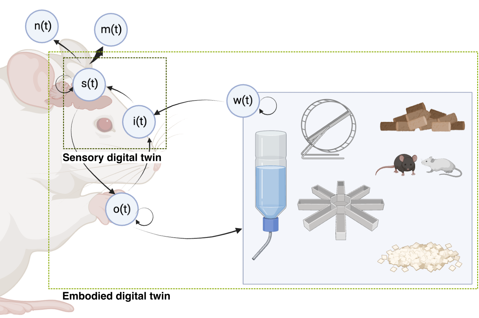
Foundation models of the brain, whole-brain simulations, and digital twins are sometimes conflated. For the purpose of this discussion, we use the following definitions (Figure 4):
Sensory digital twins seek to model an animal’s sensory systems, potentially with auxillary task-relevant inputs such as cognitive and motor state, at the level of representations. These are the topic of this section.
Embodied digital twins seek to model an entire animal, including its sensory, cognitive and motor systems, its body, and its relationship to the environment. An embodied digital twin could contain a sensory digital twin. We cover embodied digital twins in Section 3.
Biophysically detailed models seek to model nervous systems from the bottom-up, with detailed simulations that may include biophysically detailed neuron models and connectomes. These are covered in Section 4.
Foundation models of the brain are AI models trained at a large scale, usually using self-supervised or unsupervised learning, that seek to find good representations of neural data–which may include single-neuron data, local field potentials, electrocorticography, EEG, fMRI, and optionally behavior. Note that foundation models are a general approach that could be used as past of the construction of the types of models above. They are the subject of Section 3.3.2.
The boundary between these types of models can be diffuse, but we use them here to facilitate concrete discussion. We use the following working definition for a sensory digital twin:
They are models that learn the relationship between stimuli and neural responses \(f(i(t)) \to s(t)\), where \(i(t)\) are stimuli and \(s(t)\) are neural response vectors. Sensory inputs can potentially include visual, auditory, somatosensory, proprioceptive or olfactory inputs.
They are typically trained directly on single neuron response data, either from scratch or via fine-tuning after task-relevant pre-training, such as image recognition.
They are optimized to maximize their success at predicting neural responses, using metrics such as \(R^2\) or log-likelihood [86].
They are primarily focused on predicting responses of neurons to sensory stimuli, although they can also leverage other task-relevant inputs such as cognitive state, or motor inputs such as eye position and pupil dilation.
They use scalable architectures such as convolutional neural networks (CNNs), transformers or state-space models (SSMs) that can leverage arbitrarily large datasets.
As their predictive accuracy and ability to generalize improves, these models capture more and more of the computational principles and representations that underlie biological perception.
Much recent work has focused on the building of digital twins of the primary visual cortex (V1) in mice [66, 68, 87, 88, 89, 90] and macaques [89, 91, 92]. This line of work has been extended to other visual macaque area V4 [67, 93, 94, 95, 96, 97]. This follows from a long tradition, predating the deep learning revolution, of characterizing visual systems through nonlinear systems identification methods [86, 98, 99, 100, 101, 102]. Although vision is by far the most well-studied modality, [103] have developed digital twins for auditory processing in rats and ferrets, and [104] for proprioception in the macaque brainstem and somatosensory cortex.

As a concrete example of how one might build a digital twin, consider a deep CNN trained from scratch on a large-scale dataset consisting of thousands of paired natural images (sensory stimuli) and simultaneous neural responses collected from thousands of neurons in the primary visual cortex (V1) of multiple mice (Figure 5). The model receives as input an image, and optionally a set of auxiliary information, including the mouses eye position and pupil dilation. The core of the model is a CNN which finds a good latent representation of the visual input; neuron-specific readouts perform a linear weighting of the latents to predict the response of each neuron. The entire network is trained end-to-end to predict neuron responses using a learning objective such as Poisson likelihood or mean-squared error.
Once a core has been trained on a sufficient amount of neural data, the hope is that it can be used as a proxy for sensory systems in a wide range of scenarios: that it captures a kind of average sensory system. An ideal core would transfer to other unrecorded neurons in the same area and same animal; to neurons in other animals; to stimuli outside the input distribution; or even to other species. It could also serve as a basis for understanding higher-level areas in the same species.
Feasibility of building digital twins
Despite 70+ years of research on the primary visual cortex (V1) [106], and consensus by neuroscientists that it is one of the most well-understood brain areas, Olshausen & Field [107] famously estimated that we still do not know what 85% of V1 is doing. They attributed this to a combination of nonlinearities, low spike rates, inaccessible neurons, and low variance accounted for. Now that large-scale recordings and powerful nonlinear function approximators are ubiquitous, is it feasible to capture the response properties of all neurons in V1–or perhaps the entire sensory system–using digital twins? How much data would be needed to train models to capture its variance?
One way to answer this question is to examine and estimate scaling laws for digital twins of the visual system, drawing from existing results in the literature. Several studies that have built digital twins of visual areas in response to natural images and movies have documented the average performance of their models in predicting held-out data. A select few [66, 87, 89, 94, 97] have systematically varied the amount of training data that goes into fitting the models and measured goodness-of-fit on a held-out dataset. We aggregated all of these studies in Figure 6, rescaling the goodness-of-fit to fraction of explainable variance explained (FEVE) to allow consistent comparison across all studies (see Methods for details).
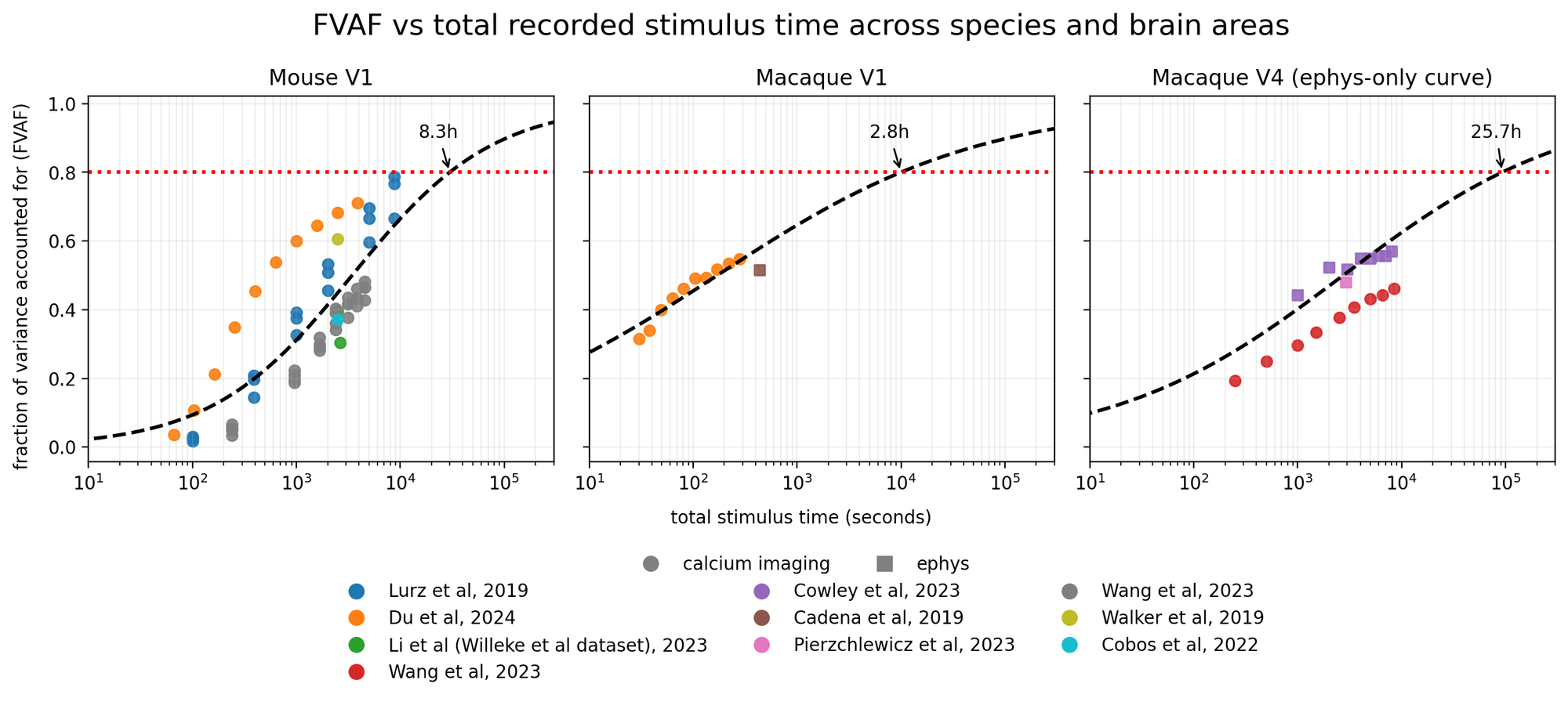
The shape of these curves across three areas (mouse V1; macaque V1; macaque V4) is well-described by a sigmoid in log-recording time:
\[\textrm{FEVE} = \sigma(a \log(t) + c)\]
We extrapolated these scaling laws to estimate the total amount of recording time necessary to obtain an average validated fraction of explainable variance explained (FEVE) across all recordings greater than 80% for their training distribution. This yielded a projected recording time to 80% FEVE of 3 hours in macaque V1, 8 hours in mouse V1, and 26 hours in macaque V4.
We emphasize here that these scaling laws were derived from presenting natural images, except for [66], which used natural movies, and thus only represent one potential stimulus class; that the stimulus sets and preprocessing steps were different across the different studies, such that the results are not directly comparable across studies; and that the distributions of stimuli were generally similar across train and test sets, thus representing a best-case scenario during evaluation–for out-of-distribution model evaluation see [66]. Despite these caveats, it is interesting and noteworthy that digital twins appear to follow similar scaling laws across a range of studies [87, 109].
At face value, this indicates that obtaining good digital twins of single neurons in the visual system to natural images is at the edge of feasibility given current technological limitations with acute recording technologies like Neuropixels (maximum recording length of ~3-4 hours in a single session). In particular, in macaque V4, one would likely need chronic electrophysiological recordings–or recording for multiple days with a technology, like calcium imaging, that allows one to stitch recordings–to get to the projected 26 hours of recordings. We note, however, that some stimulus types can be more informative than others [110, 111], and that closed-loop techniques could significantly improve upon these scaling laws [67, 68, 112].
Scaling laws for cores vs. readouts
The scaling laws in the previous section focused on the feasibility of building a digital twin of a single neuron, which depends on effectively learning the readout. However, the artifact we really care about is the core, a distillation of the processing within an area, which can be learned by stitching data together across neurons, animals and sessions. In the particular implementation of digital twins we discussed so far, the tuning of the neurons is embedded in a latent space that learns the non-linear relationships between neural responses and sensory input and other variables like motor responses. Each neuron’s response is then modeled as a linear readout of the core, where the readout is learned separately for each neuron. How do cores scale with data? In particular, how much data do we need to learn good cores, and how does this affect the scaling laws for learning accurate models of individual neurons?
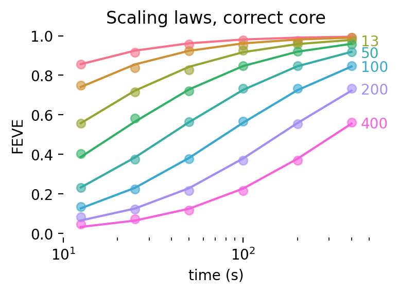
To disentangle core and readout scaling, we turn to simulations. We start with a simulation where the correct core is known a priori: it is simply the identity function over the inputs. In this case, all we need to learn are the weights of the readouts, and we’re in a situation equivalent to multivariate Poisson regression. We generate random design matrices and random weights for linear-nonlinear-Poisson (LNP) neurons, estimate maximum a posteriori weights (MAP) under Tikhonov regularization constraints, and estimate the FEVE in a validation dataset.
We find that scaling laws for these models are qualitatively and quantitatively well explained by a sigmoid as a function of log recording time and log number of parameters in the readout:
\[\textrm{FEVE} = \sigma(a \log(t) + b \log(\textrm{readout params}) + c)\]
On a log-linear scale, increasing the dimensionality of the core, and consequently of the readout weights, shifts the curves to the right, as more data is needed to fit the readout weights. We derive a mathematical expression for the functional form of scaling laws for linear regression which matches the log-sigmoid scaling laws we empirically find here (see Appendix).
What happens when the core is incorrect? Imagine, for example, that a neuron in V1 is selective for the sign of an edge, but displays some translation invariance. In other words, this neuron displays properties that place it somewhere between the classic orientation-and-phase-selective simple cell and a phase-invariant complex cell. If we tried to learn a linear mapping from an image’s luminance values to this neuron’s responses, we would not be able to fully account for the responses of the neuron no matter how much data we train on; we’d need a nonlinear mapping.
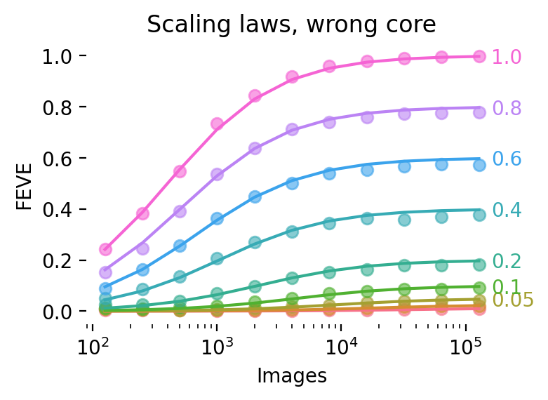
We simulate this effect by partitioning the design matrix into two components: one part which is known, and for which we can estimate linear weights as before; and a second component which is unknown, and for which we cannot estimate weights by construction. The effect is shown in Figure 7. The takeaway is that using the wrong core scales down the entire curve, capping the maximum attainable FEVE. A secondary effect is that using a bad core delays learning, as the unaccounted component of a neuron’s response decreases its effective signal-to-noise ratio.
These effects are captured by the following scaling law:
\[\textrm{FEVE} = R^2_{core} \sigma(a \log(t) + b \log(R^2_{core}) + c)\]
Note that this scaling law predicts that with bad cores, learning is delayed indefinitely. We obtain excellent fits with three free parameters (R2 > .999 in both cases) with this functional form.
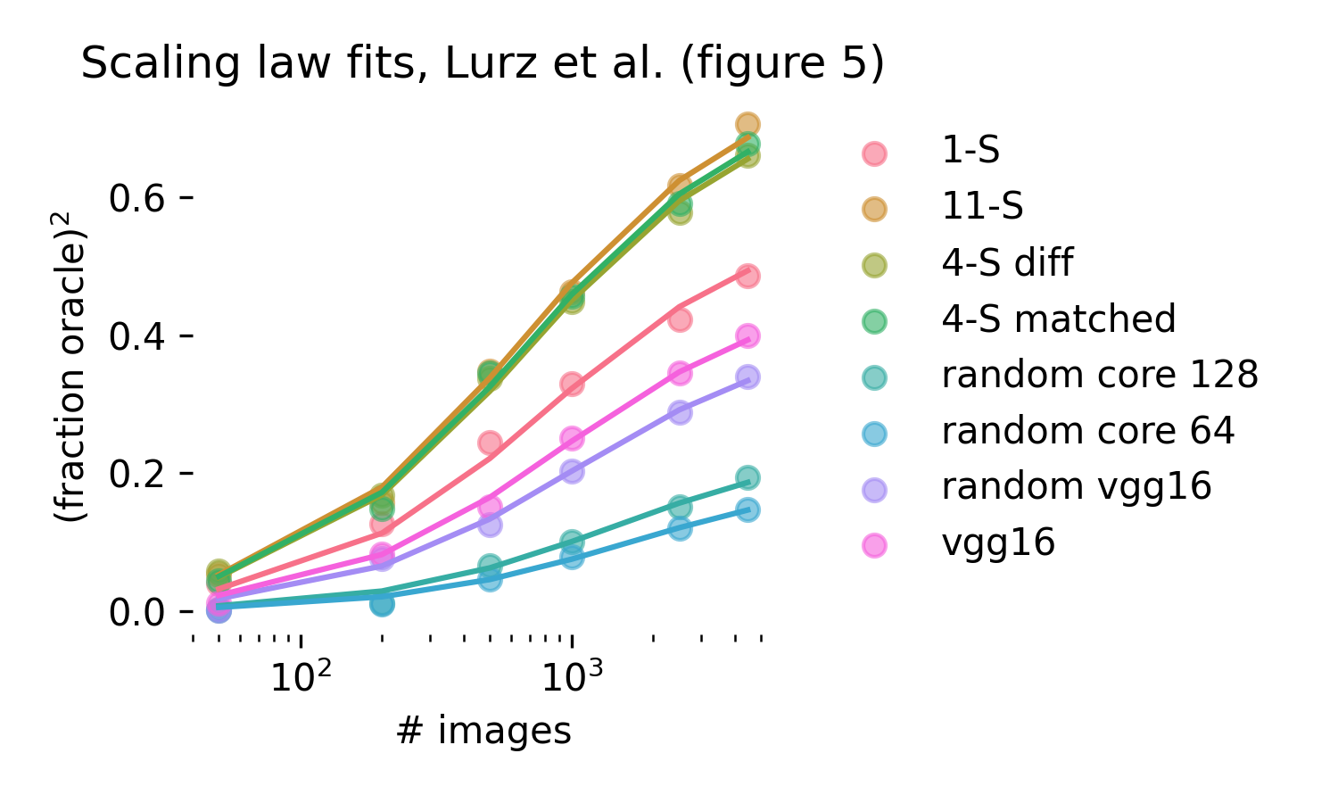
Does real neural data follow the same scaling laws as these simulations? We turn to Lurz et al. (2021) [87] to verify that this is the case. Their figure 5 explores how single neuron fits in the mouse V1 scale with data for different fixed cores that are matched to mouse V1 to varying degrees. This comparison corresponds exactly to our wrong core simulations, and indeed we obtain excellent fits using the same functional form we used in simulations (R2=.997).
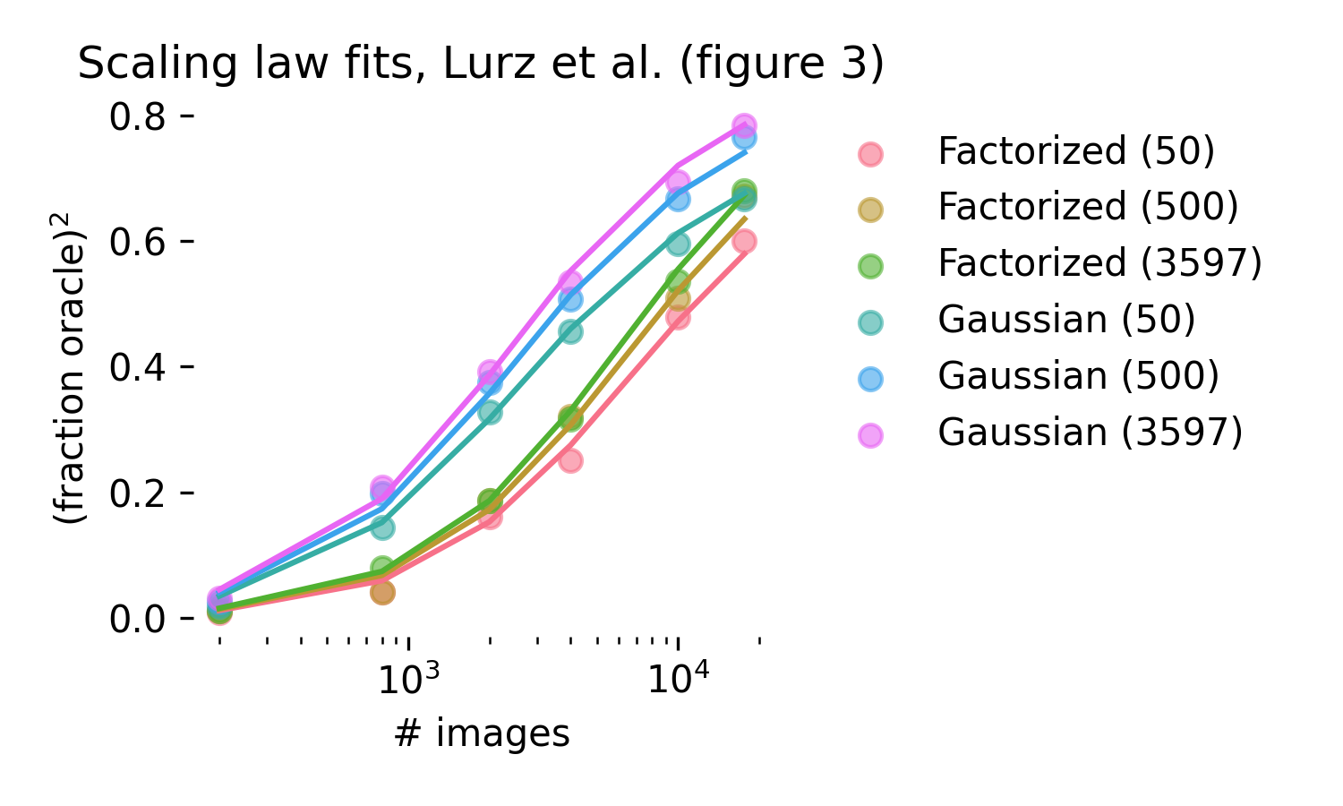
What happens when cores are learned? We assume that the maximal attainable R2 by a core scales similarly to how single neuron training scales, but with different scaling parameters1:
\[R^2_{core} = \sigma(a_{core} \log(t \cdot \textrm{neurons}) + c_{core})\]
Figure 3 in Lurz et al. (2021) quantifies how single neuron fits scale as more data is used to train both the core and the readout, allowing us to test this functional form. We obtain excellent fits, R2 = .996 for a 5 parameter scaling law. Importantly, scaling laws for the core are far slower than for the readout; the parameter a is estimated to be 1.13, while \(a_{core}\) is estimated at .15. The core, in these model fits, is far more data hungry than the readout, but better cores can be learned by pooling data together across experimental sessions and animals–that is, by sampling different neurons from the same area.
Thus, scaling curves for individual neurons are the product of the effect of the maximal variance attainable by the core and the readout scaling law for that neuron [113]. We summarize how different factors will affect the scaling law for a single neuron:
Different readout mechanisms. Higher dimensional dense readouts will shift learning curves right, and lower dimensional readouts will shift learning curves left, provided they don’t discard crucial variance in the core. Sparse readouts, whose scaling should depend on the number of non-zero readout parameters rather than total parameters, are an underexplored but promising avenue to increase readout efficiency [89, 94].
Different cores. Fixed, suboptimal cores cause two effects: scaling learning curves down, and moving learning curves to the right. Cores should be learned from the data. Data-efficient architectures trained on large numbers of images and neurons can shift the scaling curves to the left. Congruent with this, Wang and colleagues [66] showed that a more powerful core trained on eight mice mice and around 66,000 neurons could reach the same performance with 16 minutes of recording time in a new mouse than with 76 minutes of data if trained on the neurons from the new mouse alone.
Different areas. Areas higher up the visual hierarchy, which accumulate multiple stages of nonlinear processing, likely require learning a more elaborate core. This makes it more challenging to learn the response function of a single neuron. A promising research avenue is to use a core initialized from a lower-level area to bootstrap learning of a core for a higher-level area, and to use deep learning architectures that can better model internal brain states [114], which are more dominant in areas higher up in the visual hierarchy.
Different estimation schemes for maximum variance explainable: Misestimating maximum explainable variance should cause a multiplicative scaling of learning curves.
Different SNR thresholds for inclusion: Including neurons with low spike rates is expected to drag average prediction performance down, shifting learning curves to the right. Using low SNR modalities like single-photon imaging should have the same effect [97].
Different stimulus sets. A less well-explored phenomenon is the effect of different types of stimuli [110]. Using spatiotemporally varying stimuli (movies) rather than static stimuli (images) is expected to shift learning curves to the right, as more parameters are needed to describe the readout.
While we have focused on scaling laws for single neurons, the framework proposed here allows one to estimate the quality of a core: the asymptotic \(R^2\) of a core, the maximum that could be obtained if one had access to infinite single neuron data, can be extrapolated from fitting single-neuron scaling laws. Obtaining a high ranking on this metric is a prerequisite for making a claim that a digital twin has been achieved. However, it is by no means the only metric that matters [115, 116, 117].
Given the bulk of the evidence, we tentatively conclude that it should be feasible to learn good models of individual neurons in visual areas of mice and macaques using single session, acute recordings (2-3 hours) by distilling rich cores from multiple sessions and animals. We leave open the possibility that higher-level areas may require chronic recordings to go past the 3-hour barrier [118]. Of course, such models will be static snapshots stitched together from multiple animals; dynamic models incorporating learning, or personalized models are likely to still require a larger amount of data, although it’s difficult to forecast at this time. While we have not established that this holds for modalities other than vision, we see no obvious additional technical barriers to doing this for audition; somatosensory and olfactory maps will likely require better, more comprehensive actuators than is currently feasible.
Although macaques have been used as stand-ins for humans in vision research for decades, and there is high homology, their visual representations and brain organization do differ from humans [119]. Furthermore, the human visual cortex is rarely recorded with electrophysiology, although this may change through a push toward cortical visual prosthesis [120]. Fine-tuning macaque pretrained models on human data collected noninvasively is one potential route to human digital twins. This also appears more feasible than directly training on fMRI data, where each voxel averages over tens of thousands of neurons, and where a wide variety of models can account for the data equally well [121].
Beyond vision, audition is greatly expanded in humans and specialized for language. Given the push toward novel speech neuroprosthesis [122, 123], and the sustained interest in understanding audition due to its relationship to language [124], it seems plausible that human auditory cortex data will be plentiful enough in the near future to build a digital twin [125] directly from human data, although it could benefit from pre-training on macaque auditory cortex. This is in addition to complementary advances in noninvasive decoding from auditory and speech-related areas [126, 127, 128].
Feasibility of transferring robustness from brains to models
We have seen that it’s practically feasible to build digital twins that accurately predict neural responses within their training distribution. Since primates and humans are robust to out-of-distribution shifts, and they are not sensitive to adversarial examples [44, 46, 47, 129, 130, 131], it would stand to reason that distilling neural data should lead to adversarially and distributionally robust neural networks. If this was the case, one could potentially use these robust digital twins either as adversarially robust networks for classification purposes, or as a means of reverse engineering adversarial robustness.
To the best of our knowledge, a direct approach–simply training a neural network to imitate neural data at scale and testing its adversarial robustness–has not been tried. However, several references instead use neural data to regularize networks trained for image classification. They report that regularization with neural data leads to higher adversarial or distributional robustness in the domain of natural images (Table 2 with summary of results). We refer to these methods collectively as neural data augmentation (NDA). These prior results give valuable insight into whether distilling robust representations from neural data to digital twins is feasible.
| Paper | Neural dataset | Regularization method | Target network | Evaluation dataset | Attack Type | Accuracy gain vs baseline |
|---|---|---|---|---|---|---|
| [49] | Responses from 8k mouse V1 neurons obtained with 5.1k grayscale ImageNet images | Cosine Similarity Matching loss | ResNet-18 | Grayscale CIFAR-10 | Gaussian noise (\(\sigma = 0.08\)) | +22.5% |
| ResNet-34 | Grayscale CIFAR-100 | Gaussian noise (\(\sigma = 0.08\)) | +12.9% | |||
| [132] | Responses from 188 macaque IT neurons obtained with 2880 grayscale HVM images | Centered Kernel Alignment (CKA) loss | CORnet-S | HVM (IID) | PGD \(L_\infty (\epsilon = 0.001)\) | +20.9% |
| CORnet-S | HVM (IID) | PGD \(L_2 (\epsilon = 0.25)\) | +13.3% | |||
| CORnet-S | COCO (OOD) | PGD \(L_\infty (\epsilon = 0.002)\) | +11.1% | |||
| CORnet-S | COCO (OOD) | PGD \(L_2 (\epsilon = 0.2)\) | +9.6% | |||
| [50] | Responses from 102 macaque V1 neurons obtained with 450 naturalistic textures and noise samples | Biologically-constrained V1 front-end (VOneBlock) | ResNet50 | ImageNet | PGD (high strength) | +37.1% |
| CORnet-S | ImageNet | PGD (high strength) | +36.4% | |||
| AlexNet | ImageNet | PGD (high strength) | +18.1% | |||
| [51] | Responses from 458 macaque V1 neurons obtained with 24075 ImageNet images | Multi-task learning with macaque V1 response prediction | VGG-19 | TinyImageNet-TC | ImageNet-C corruptions (without blur) | +9.0% |
Despite these promising results, we don’t have a current theory for why NDA networks are robust, and if they could ever be competitive with state-of-the-art defenses. Some studies suggest that low-frequency features can to some extent enhance robustness [133], and NDA might help learn better features more generally. The most successful class of defense against adversarial attacks remains adversarial training together with massive data augmentation [47]. This relies on training a network on adversarial examples. Yet, NDA only accounts for responses to clean examples, not to adversarial examples. Why does training on clean examples improve the performance of neural networks on corrupted (adversarial, out-of-distribution) examples?
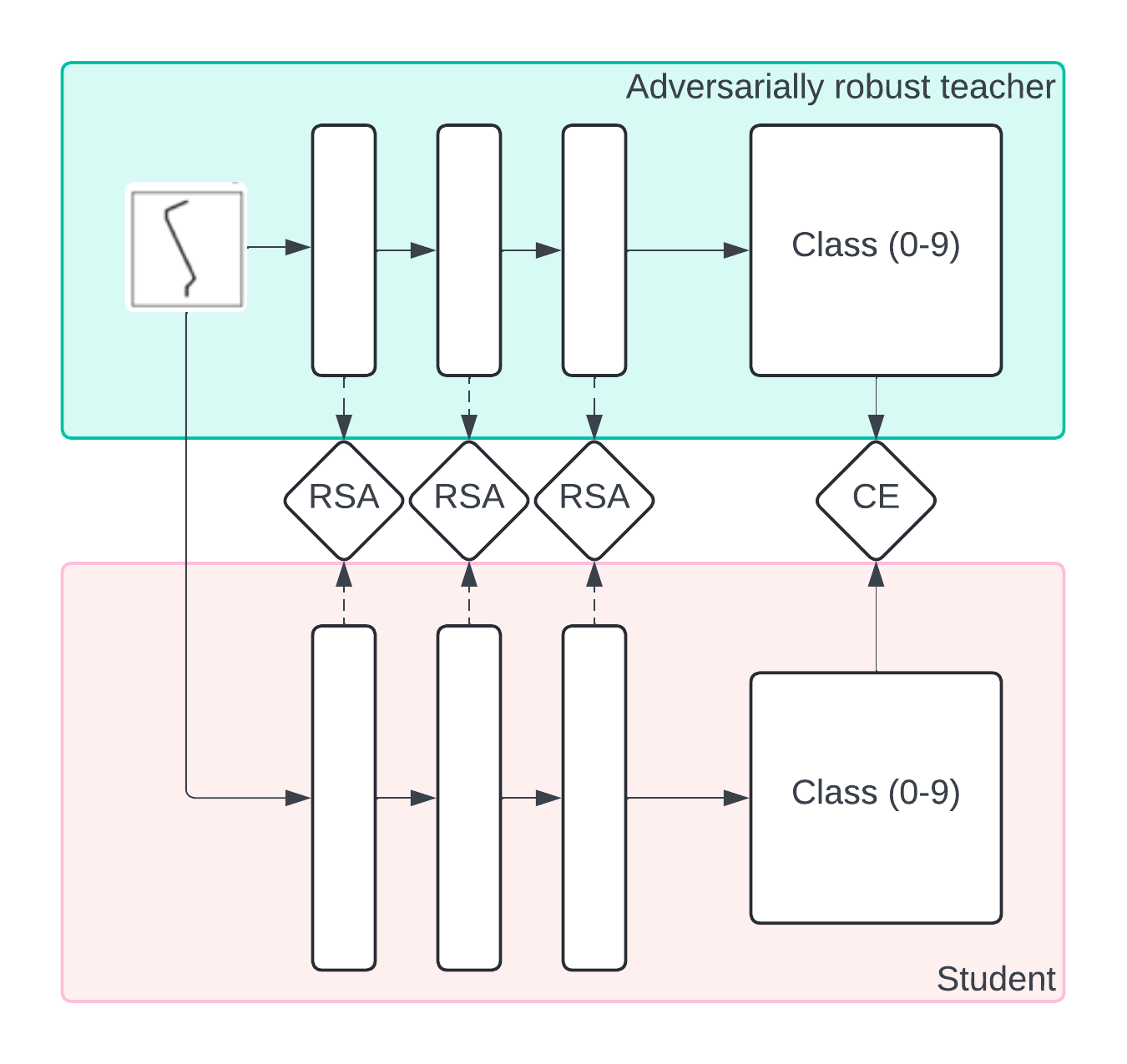
To make progress on these questions, we turn to teacher-student simulations, in which we test whether training a student to imitate a robust teacher leads to robust representations. Here, the robust teacher is a stand-in for the brain; however, unlike real brains, we can generate arbitrary amounts of data from the teacher.
We leverage MNIST-1D, an algorithmically generated dataset that allows us to generate arbitrarily large numbers of training examples and train many networks very rapidly. We first train a small three-hidden-layer CNN adversarially on large amounts of generated data, obtaining a robust network. We then use this robust network as the teacher for a student network. We consider two scenarios:
The student is only trained on the teacher’s labels. This is conceptually similar to the business-as-usual scenario of training only on labels.
The student is trained on the teacher’s labels and intermediate activity. We compute representational similarity matrices and match the intermediate activity of the teacher and student at their three convolutional layers on clean examples–we refer to this as a representational similarity analysis loss (RSA). This is conceptually similar to using neural data augmentation to match intermediate activations of teacher and student [49].
Both clean accuracy and adversarial accuracy under an adversary are noticeably increased under these scenarios across all dataset sizes (Figure 10). The representation similarity loss forces the intermediate activations to match those of the robust network, essentially forcing the student to follow not just the labels of the robust network but also its strategy, boosting in-distribution and adversarial generalization.
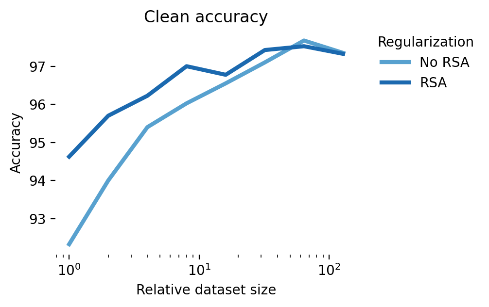
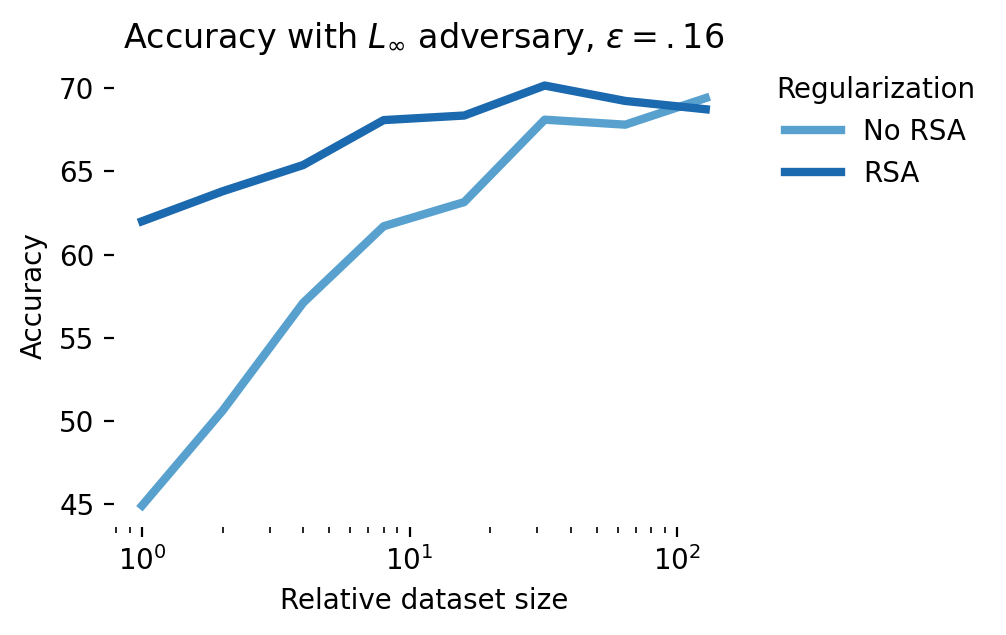
These results are promising and in line with the NDA literature. To move beyond a proof-of-concept, however, and positively impact AI safety, we’d need to show that it’s possible to do better than the state-of-the-art, adversarial training. The results shown in Figure 11 show that while NDA does better than standard training, adversarial training offers a more direct route to robust students: at the smallest dataset size, with an \(\epsilon=0.16\) adversary, no augmentation gives 45% accuracy, RSA gives 62% accuracy, and adversarial training obtains 68%. Combining RSA and adversarial training in these simulations gives a small but consistent performance boost of up to 1% over adversarial training only. In the regime of scaling laws for adversarial training, a 1% improvement in adversarial robustness could be matched with a ~2X increase in FLOPs [47].
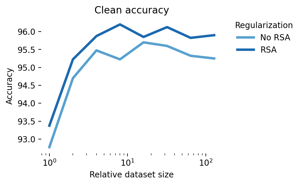
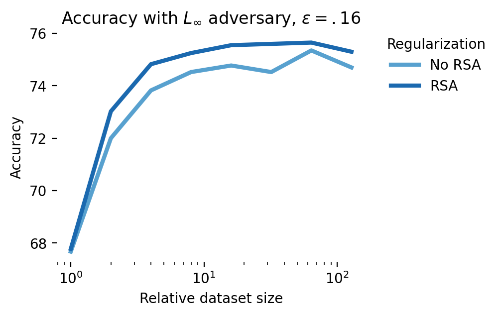
We extended these simulations to CIFAR-10 (Figure 12). Here again, aligning latent representations with those of a robust teacher leads to an improvement in robustness. However, this improvement in robustness is diminished and eventually eliminated when activations are noisy. This shows a potential role for digital twins trained on neural data in improving adversarial robustness: a digital twin trained at multiple stages of a sensory hierarchy can be used to essentially denoise latent activations [49].
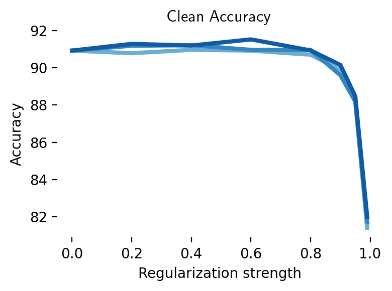
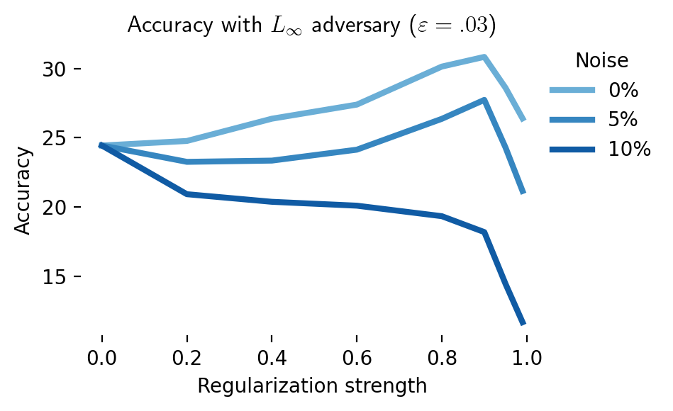
These results show there is a regime in which data from the brain could help adversarial robustness, especially if future brain augmentation methods can leverage brain data more effectively [134]. It does, however, highlight a gap in the literature: most papers surveyed here compare brain-augmented training against vanilla non-robust networks, not robust networks. The latter comparison is, in our opinion, more relevant for AI safety applications. Direct engagement with state-of-the-art benchmarks [135] is desirable. Furthermore, if the solution to adversarial examples lies in the brain, one would want to measure how adversarial examples, as opposed to clean examples, affect representations at different levels in the sensory hierarchy [46].
While these results indicate a rather narrow direct path for neural data directly improving robustness in artificial neural networks, we remain optimistic that better understanding the computational and information processing principles of how robust representations are formed in the brain could inspire new adversarially robust algorithms [48, 136].
Evaluation
Digital twins of perceptual systems could potentially contribute towards safer AI systems by:
Allowing one to predict a subject’s perception in reaction to a physical stimulus, which could facilitate human-AI interactions
Distilling more robust representations than is currently feasible with data augmentation and adversarial training alone
Enabling virtual and closed-loop experiments that tease apart the circuit mechanisms, inductive biases, and representation geometry underlying robust perception (see also Section 8 for a discussion on mechanistic interpretability)
Scaling laws indicate that building digital twins that account for a large fraction of the explainable variance in a particular area is likely feasible with current technology in model species, while the path to scale up to humans remains more speculative. The data used to train digital twins may be useful to enhance adversarial robustness in existing neural networks; furthermore, digital twins as an intermediate step to denoise activations in neural data augmentation may lead to more effective regularization than the direct approach of using noisy neural data directly as a regularizer. To move beyond proofs of concepts, we identify one bottleneck, the measurement of neural responses to adversarial stimuli. We also single out better understanding the geometry of human robustness to adversarial stimuli using large-scale psychophysics as an important bottleneck to improving adversarial robustness [47].
Opportunities
Create large-scale neural recordings from sensory areas in response to rich spatiotemporal stimuli
Focus on bringing down the required single-neuron recording times to reach high FEVE within a 3-4 hour recording session
Improve efficiency of transfer function estimation by learning compact cores, or by using sparse readout mechanisms
Scale promising chronic recording technologies to allow recording beyond the 3-4 hour single-session limit
Build sharable, composable digital twins of sensory systems
Measure and report scaling laws on an apples-to-apples basis, for both single-neuron transfer function estimation and the ceiling attainable by a core
Share pretrained models in a standardized format to bootstrap the creation of fine-tuned models
Expand beyond vision to other modalities, including audition and somatosensation and more motor variables
Build robust digital twins
Measure in-vivo neural responses to adversarial stimuli in a closed-loop fashion
Build robust digital twins through adversarial training and anchoring to measured neural responses to adversarial stimuli
Estimate the geometry of adversarial robustness in humans through large-scale, online psychophysics
Track and report robustness of digital twins to adversarial and out-of-distribution stimuli across a range of relevant attack dimensions (e.g. \(L_\infty\) and \(L_2\) robustness, distributional shifts)
Compare against state-of-the-art defenses rather than against non-robust training
Box: Scaling trends for neural recordings
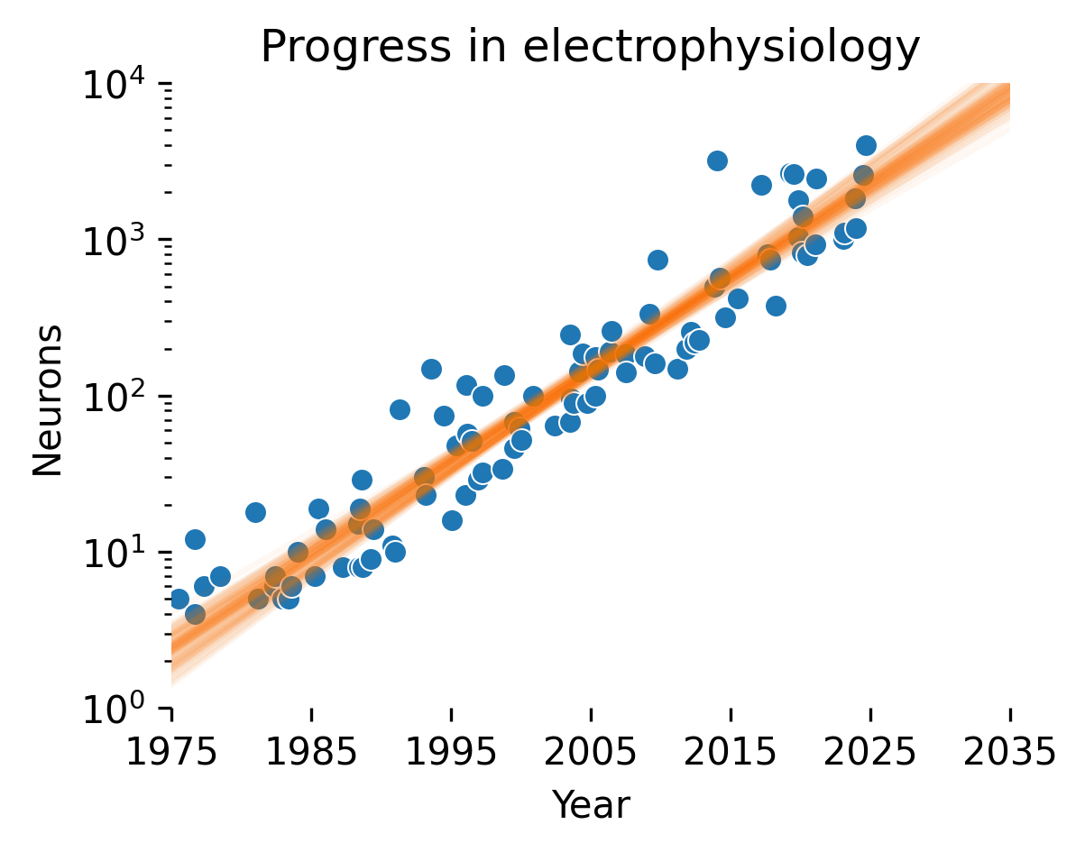
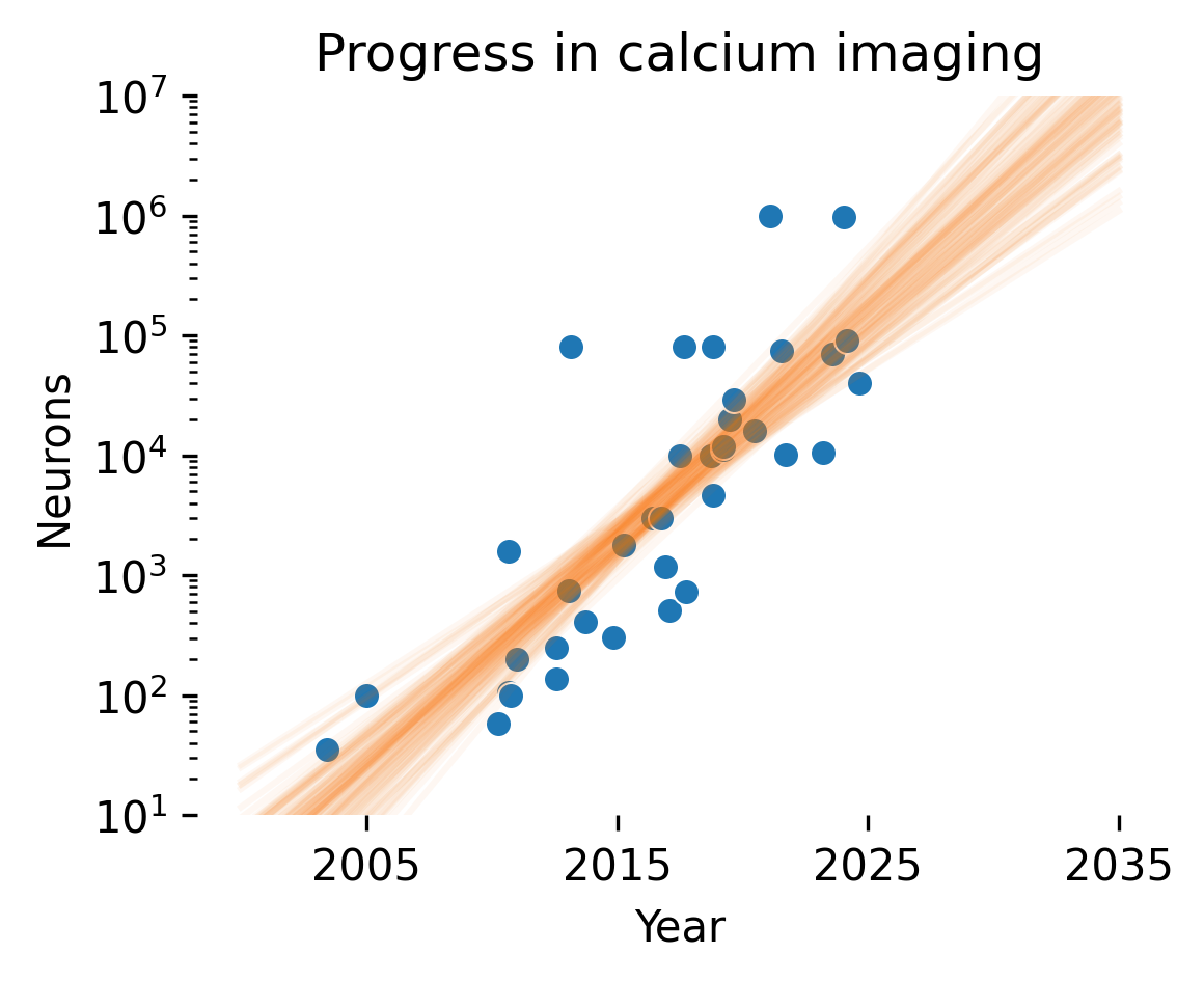
Many of the approaches to NeuroAI safety that we discuss are dependent on the continued creation of ever-larger datasets with more capable recording techniques. For instance, under log-linear scaling laws, to obtain linear improvements in performance over time, one would need to obtain datasets that grow exponentially over the same time. Stevenson [137] first documented a Moore’s-law-like relationship for recording capabilities in electrophysiology, estimating that simultaneously recorded neurons double every 7 years; Stevenson recently updated his estimate at 6 years. Urai et al. [138] extended these results to calcium imaging; while the growth was not quantified, the trend pointed toward exponentially faster improvements in calcium imaging.
We extended these results to update these scaling trends using an LLM-based pipeline to identify relevant papers (see methods for details) and joining them with previous databases collected by Stevenson and Kording and Urai et al. Fitting a Bayesian linear regression to the log number of neurons for recordings after 1990, we obtained an estimated 5.2±0.2 year doubling time for electrophysiology and 1.6±0.2 year doubling time for imaging.
Out of the 10 electrophysiology studies reporting the largest simultaneous neuron numbers recorded, 9 were performed with multi-shank Neuropixel recordings. Light bead microscopy is currently the state-of-the-art for calcium imaging [139]. If current trends continue, we predict that in 2035, 10,000 neuron electrophysiological recordings will be commonplace, whereas calcium imaging should reach 10M neurons. A concerted investment in neurotechnology could break these incremental trends, in particular for electrophysiology.
These trends are important to contextualize how digital twins will evolve; indeed, scaling laws for digital twins suggest linear improvements in our ability to predict neural activity with exponential increases in channel count. However, this analysis does not assess the signal-to-noise ratio (SNR) of different recording technologies. While this is more or less constant in electrophysiology, SNR can vary widely in imaging depending on the amount of out-of-focus light and the size of the focus area (e.g. one-photon vs. multiphoton imaging approaches). Thus, it’s likely that we’ll see optimizations in terms of signal-to-noise ratio rather than increasing channel count as we approach whole-brain coverage with imaging.
We consider a single scaling parameter \(a_{core}\), but one could easily extend this framework to have different scaling parameters for, e.g. recording time, number of neurons, number of animals, entropy of the stimuli, etc.↩︎